TCT

Hi Andres!

Based on our investigation, here is the answer: “

• If you’re asking if the Tasseled Cap exists for PlanetScope data, it does not. If you’re asking how to derive the Tasseled Cap then this paper will help to get the transformation coefficients. The paper includes Gram-Schmidt orthogonal transformation for RapidEye data which can be also applied in the same way to SuperDove data.
   
• A way to get yourself a fixed orthogonal transformation of Planetscope data is to use PCA (Principal Component Analysis):
  1. Get a good variety of PlanetScope scenes (same sensor type, e.g. SuperDove only),  
  2. Sample pixels from the scenes (or use full scenes)
  3. Throw them into PCA
  4. PCA gives you back the Eigenvectors (these Eigenvectors can act as your fixed orthogonal transformation coefficients, but they are not the Tasseled Cap features (but might be as useful as them)
   
•  Here is an example of a PCA on scenes of the Palouse region (USA) and Koethen, Germany. The area in Palouse and Koethen are highly agricultural regions (diverse wheat crops). 
  
  The Eigenvectors can be used as a fixed orthogonal feature space, i.e. applying the eigenvectors (called *_coeff in the first attached csv) to any other (new) image, e.g. like

PC1 = coastal_blue_coeff * Coastal_blue + blue_coeff* Blue + green_i_coeff * Green_I + green_ii_coeff * Green_ii + yellow_coeff * Yellow + red_coeff * Red + sentinel_red_edge_i_coeff * RedEdge + nir_coeff * NIR

PC2 = ....

where *_coeff are the coefficients (Eigenvectors) of the PCA (e.g. in the csv file) and Coastal_blue, Blue, Green_i, ..., NIR are the pixels/bands of the image that is being transformed
 

Result is an orthogonal transformed image / an image that was transformed to the feature space of the fixed PCA. 

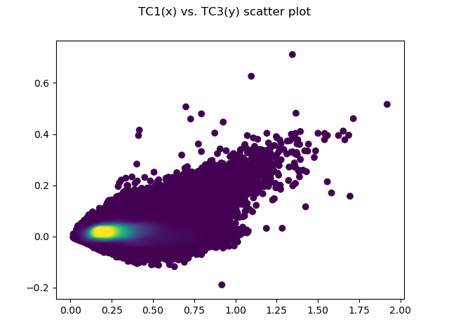
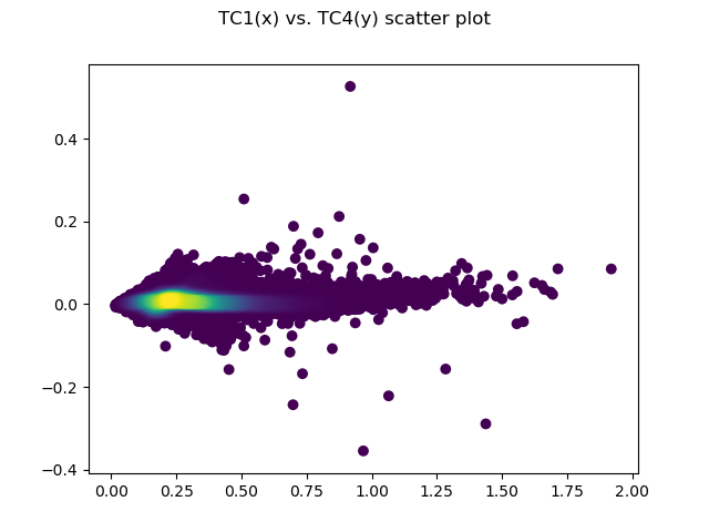
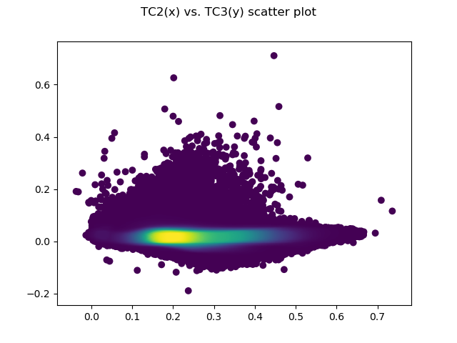
The screenshots show how the pixels of images (here the images that were used to derive the PCA Eigenvectors) fall into the new, orthogonal, fixed PCA feature space. 

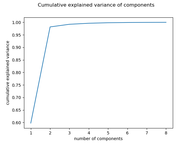
The "cumulative_explained_variance" graph shows how much variance (information) was contained in the Principal Components (that were derived from the Palouse and Koethen areas).”

Let us know if you have further questions. Have a great day!