Sticky

Open Data for Planetary Variables in Sentinel Hub

  • 26 January 2024
  • 1 reply
  • 140 views

Userlevel 2
Badge +4

Planet recently released support for delivering Planetary Variables to Sentinel Hub.  Check out this product announcement and this blog post if you’d like to learn more about what’s been released. To help you explore these new datasets and capabilities, we have also released open datasets for several of our Planetary Variables.  We’ve opened these datasets to allow for anybody to explore what this data looks like or to test workflows.

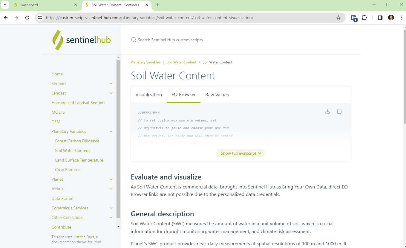
As part of this open data release, data is available for Land Surface Temperature, Crop Biomass, and Soil Water Content.  There is 4 years of data from 2019 to 2022 across 4 areas of interest in Uruguay, India, Germany, and the US.  You can explore more information about these collections here: https://collections.sentinel-hub.com/tag/planetary-variables/.  By clicking through to the specific Planetary Variables, you’ll be taken to their open data pages, such as this Soil Water Content Open Data page.

To make it simple to use these open datasets, they have been hosted in Sentinel Hub. If you don’t already have a Sentinel Hub account, you can sign up here.  As part of the 30 day Sentinel Hub trial, you can use the APIs to interact with these open datasets.  In addition, if you have a Planet account to order data with, you can also use the 30 day trial to test Sentinel Hub with your own data by using the Sentinel Hub Third Party Data Import API.

If you have any questions about how to use these, feel free to reach out here! 

Example Workflow in EO Browser

The open datasets can be explored in EO Browser or used with the Sentinel Hub APIs.

To use these datasets with EO Browser, you’ll want to follow these steps:

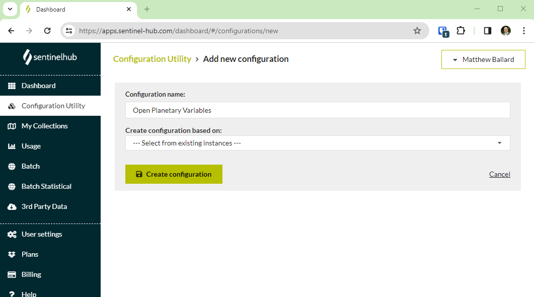
  1. Create a new configuration in your Sentinel Hub Dashboard


  2. Add a layer to the configuration and use one of the collection IDs from the open data webpages


  3. Add a custom script from our custom scripts repository.  This dictates how the Planetary Variables will be visualized.  Use one of the scripts that support EO Browser.
  4. Save the layer with the collection type set to “BYOC”, the collection ID, and the Data processing set to the custom script.
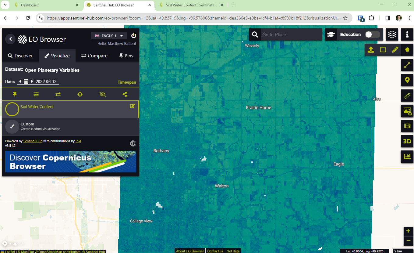
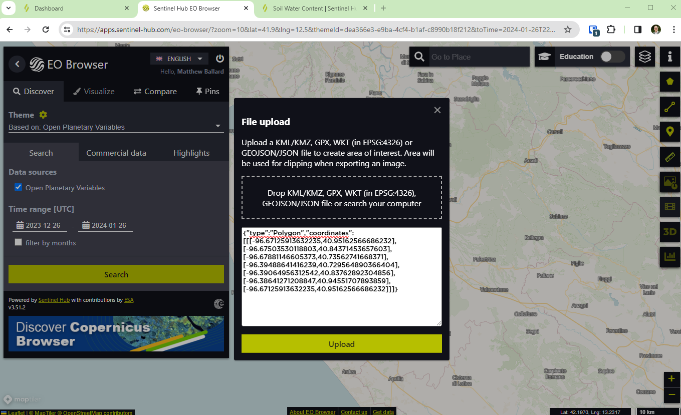
  5. From the bottom left, select open in EO Browser. In the top right of EO Browser, add the geojson boundary for one of the areas of interest (found on the open data pages). This will zoom the map to the data extent.
  6. Change the time range on the left and search for data. Select visualize to view the imagery on the map.


1 reply

Userlevel 2
Badge +4

As well, here is a Python code sample that works with the Crop Biomass open data collection:

from sentinelhub import (
DataCollection,
SentinelHubDownloadClient,
SentinelHubStatistical,
SHConfig,
Geometry,
CRS
)
from shapely.geometry import shape
import pandas as pd
import json

# Provide credentials to connect to Sentinel Hub
# https://sentinelhub-py.readthedocs.io/en/latest/configure.html#environment-variables
config = SHConfig.load()
uswest_config = config
uswest_config.sh_base_url = "https://services-uswest2.sentinel-hub.com"


# Define your Sentinel Hub Collection
collection_id = "fc844940-ecc7-49ff-b072-9f81b36ef191" # Replace with a collection ID
data_collection = DataCollection.define_byoc(collection_id)
input_data = SentinelHubStatistical.input_data(data_collection)

area_of_interest = '''{
"type": "Polygon",
"coordinates": [
[
[
-10743613.707363,
4991187.393896
],
[
-10743613.707363,
4992276.731204
],
[
-10742541.14407,
4992276.731204
],
[
-10742541.14407,
4991187.393896
],
[
-10743613.707363,
4991187.393896
]
]
]
}'''


area_of_interest = shape(json.loads(area_of_interest))

# Specifiy your time of interest (TOI)
time_of_interest = "2020-01-01", "2021-01-01"

# Specify a resolution
resx = 100
resy = 100

# Provide an evalscript
#time_series_evalscript_path = "crop_biomass.js" #using the previous eval script
#with open(time_series_evalscript_path, 'r') as file:
# time_series_evalscript = file.read()

time_series_evalscript = '''
//VERSION=3
// To set custom max and min values, set
// defaultVis to false and choose your max and
// min values. The color map will then be scaled
// to those max and min values
function setup() {
return {
input: ["CB", "dataMask"],
output: [
{ id: "default", bands: 4 },
{ id: "index", bands: 1, sampleType: "FLOAT32" },
{ id: "eobrowserStats", bands: 1, sampleType: "FLOAT32" },
{ id: "dataMask", bands: 1 },
],
};
}

const bp_ramp = [
[0, 0xfff7ea],
[0.1, 0xf3e3c8],
[0.2, 0xdad0a4],
[0.3, 0xbdc082],
[0.4, 0x99b160],
[0.5, 0x6da242],
[0.6, 0x2c952e],
[0.7, 0x008729],
[0.8, 0x007932],
[0.9, 0x006640],
[1.0, 0x005444],
];

const visualizer = new ColorRampVisualizer(bp_ramp);

let factor = 1 / 1000;
function evaluatePixel(sample) {
let val = sample.CB * factor;
let imgVals = visualizer.process(val);
return {
default: [...imgVals, sample.dataMask],
index: [val],
eobrowserStats: [val],
dataMask: [sample.dataMask],
};
}'''

# Create the requests
aggregation = SentinelHubStatistical.aggregation(
evalscript=time_series_evalscript, time_interval=time_of_interest, aggregation_interval="P1D", resolution=(resx, resy)
)

request = SentinelHubStatistical(
aggregation=aggregation,
input_data=[input_data],
geometry=Geometry(area_of_interest, crs=CRS("EPSG:3857")),
config=uswest_config,
)

# Post the requests
download_requests = [request.download_list[0]]
client = SentinelHubDownloadClient(config=uswest_config)
stats_response = client.download(download_requests)

# Parse the repsonse
# Load into a pandas dataframe
series = pd.json_normalize(stats_response[0]["data"])

# Clean up columns in the dataframe by selecting ones to remove
del_cols = [i for i in list(series) if i not in ["interval.from",
"outputs.eobrowserStats.bands.B0.stats.min",
"outputs.eobrowserStats.bands.B0.stats.max",
"outputs.eobrowserStats.bands.B0.stats.mean"
]]
# Drop unused columns and rename remaining columns
series = series.drop(columns=del_cols).rename(columns={'interval.from': 'date',
'outputs.eobrowserStats.bands.B0.stats.min': 'minimum_cb',
'outputs.eobrowserStats.bands.B0.stats.max': 'maximum_cb',
'outputs.eobrowserStats.bands.B0.stats.mean':'mean_cb'
})
# Calculate new columns
series["mean_cb"] = series["mean_cb"].astype(float)
series["date"] = pd.to_datetime(series['date']).dt.date
series["day_of_year"] = series.apply(lambda row: row.date.timetuple().tm_yday, axis=1)
series["year"] = series.apply(lambda row: row.date.year, axis=1)

series.plot(x = "day_of_year", y = "mean_cb")


Output from the sample script


Reply