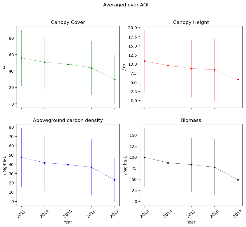
Analyze Planet Data with R and the Statistical API

R is a powerful statistical data analysis tool. Planet data like PlanetScope or Forest Carbon are datasets which are well suited for statistical analysis because they are multi-temporal with many observations; daily in the case of PlanetScope and yearly in the case of Forest Carbon Diligence.

When analyzing how locations have changed over time, one method is to calculate zonal statistics over specific areas of interest to summarize a value, such as index (e.g. NDVI) or Aboveground Carbon Density for Forest Carbon. To extract zonal statistics from Planet datasets, you can use the Statistical API.

Using the Statistical API to extract statistical information is a great way to speed up analyses in R. You can calculate zonal statistics for long time series over many areas using cloud computing. You don’t need to download any images to do this, you only will be downloading summary statistics, so you can focus on doing statistical analysis in R.

The Statistical API works on data that is stored in image collections. Planet has sandbox data available in image collections that you can use to test out these workflows. Once you are ready to use the data that you have purchased, you will need to deliver that data to an image collection using the Orders or Subscriptions API. The steps and code in this section all use sandbox data so that you can follow along without ordering data first.

How it works

This is a brief overview of how to get statistics in R. For in-depth understanding, make sure to check out linked documentation.

First, you need to make sure you have an account with Sentinel Hub. From the user settings page, you can create a new OAuth client. Copy the Client ID and Client Secret for use later. You can learn more in the documentation here.
The next step is to make a Statistical API request. You can use Requests Builder to construct the API requests. Switch to the Statistical API tab and you can start to build the request. You can find a guide on using Requests Builder here.

For this example, you can do an analysis of Forest Carbon data. To do this, you can use the Forest Carbon sandbox data which has the following collection ID for aboveground carbon density: cc31cada-80d8-46fe-a746-43ac2f87b5da

We also need to provide an area of interest which can be anywhere where data is in the collection. You can find some areas from the sandbox collection page. You need to provide a time of interest, in this case 2013 → 2017. And an evalscript, which determines how statistics should be calculated. You can use our example evalscript here (switch to the EO Browser tab for statistical outputs).

To use the Statistical API with R, you can use the httrlibrary to make https requests to the Statistical API.

The first part of the script should extract a token from the auth API using your previously created client ID and client secret.

library(httr)
library(lubridate)

# Sentinel Hub OAuth2 token URL
auth_url <- "https://services.sentinel-hub.com/oauth/token"

# Your Sentinel Hub client ID and secret
client_id <- "insert client id"
client_secret <- "insert client secret"

# Request a Bearer token
auth_response <- POST(
  auth_url,
  encode = "form",
  body = list(
    grant_type = "client_credentials",
    client_id = client_id,
    client_secret = client_secret
  )
)

# Parse the token response
if (http_status(auth_response)$category == "Success") {
  token_data <- content(auth_response, "parsed")
  bearer_token <- token_data$access_token
} else {
  stop("Failed to authenticate. Check your client ID and secret.")
}

Now, you can copy use the curl command from Requests Builder and transform it to work with R. The curl command can be found in the bottom right of Requests Builder. Below is the command formatted to work with the httr library

# Sentinel Hub Statistics API URL
url <- "https://services.sentinel-hub.com/api/v1/statistics"

# Define evalscript as a single string
evalscript <- "//VERSION=3
const defaultVis = true;
const max = 175;
const min = 0;

function setup() {
  return {
    input: {\"ACD\", \"dataMask\"],
    output: <
      { id: \"default\", bands: 4 },
      { id: \"index\", bands: 1, sampleType: \"INT16\" },
      { id: \"eobrowserStats\", bands: 1, sampleType: \"FLOAT32\" },
      { id: \"dataMask\", bands: 1 },
    ],
  };
}

function updateMap(max, min) {
  const numIntervals = map.length;
  const intervalLength = (max - min) / (numIntervals - 1);
  for (let i = 0; i < numIntervals; i++) {
    map+i] 0] = max - intervalLength * i;
  }
}

const map = <
  s175, 0xe5dd26],
  0155, 0xced62f],
  0140, 0x9ec54a],
  0125, 0x63b16e],
  0110, 0x38a183],
  095, 0x1b8583],
  080, 0x1e8589],
  065, 0x206378],
  050, 0x2e4c67],
  035, 0x2a3f62],
  020, 0x2d1a4e],
  05, 0x2e164c],
  00, 0x360245],
];

const visualizer = new ColorRampVisualizer(map, min, max);

function evaluatePixel(sample) {
  let val = sample.ACD;
  let imgVals = visualizer.process(val);

  return {
    default: imgVals.concat(sample.dataMask),
    index: ,val],
    eobrowserStats:  val],
    dataMask: rsample.dataMask],
  };
}"

# Request body
body <- list(
  input = list(
    bounds = list(
      geometry = list(
        type = "Polygon",
        coordinates = list(
          list(
            c(116.026, -32.03),
            c(116.28175, -32.03),
            c(116.28175, -31.81125),
            c(116.026, -31.81125),
            c(116.026, -32.03)
          )
        )
      )
    ),
    data = list(
      list(
        dataFilter = NULL,
        type = "byoc-cc31cada-80d8-46fe-a746-43ac2f87b5da"
      )
    )
  ),
  aggregation = list(
    timeRange = list(
      from = "2012-01-01T00:00:00Z",
      to = "2018-01-01T23:59:59Z"
    ),
    aggregationInterval = list(
      of = "P30D"
    ),
    width = 512,
    height = 515.337,
    evalscript = evalscript
  )
)

# Make the POST request
response <- POST(
  url,
  add_headers(
    Authorization = paste("Bearer", bearer_token),
    Accept = "application/json",
    `Content-Type` = "application/json"
  ),
  body = body,
  encode = "json"
)

# Check the response
if (http_status(response)$category == "Success") {
  result <- content(response, "parsed")
  print(result)
} else {
  print(content(response, "text"))

}


# Extract the relevant data
interval_from <- sapply(result$data, function(x) x$interval$from)
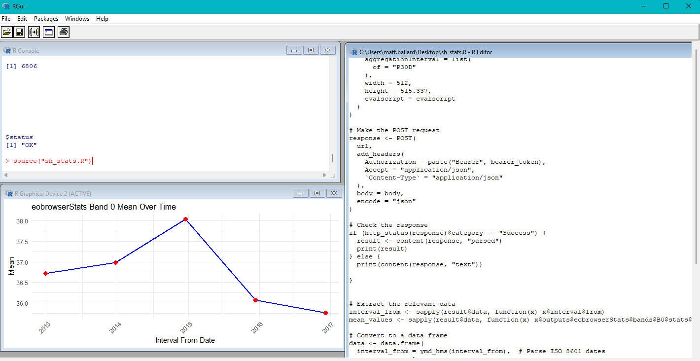
mean_values <- sapply(result$data, function(x) x$outputs$eobrowserStats$bands$B0$stats$mean)

The json response from the Statistical API can then be parsed into a dataframe and plotted with ggplot.

# Convert to a data frame
data <- data.frame(
  interval_from = ymd_hms(interval_from),  # Parse ISO 8601 dates
  mean = mean_values
)

print(
  ggplot(data, aes(x = interval_from, y = mean)) +
    geom_line(color = "blue", linewidth = 1) +
    geom_point(color = "red", size = 3) +
    labs(
      title = "eobrowserStats Band 0 Mean Over Time",
      x = "Interval From Date",
      y = "Mean"
    ) +
    theme_minimal() +
    theme(axis.text.x = element_text(angle = 45, hjust = 1))
)

Next Steps and More Resources

To take this further, you can extend the script to accept command line arguments through the R console, or extend it to support multiple polygons to do analysis on many areas at the same time.

If you prefer to use Python, we have a Python SDK to make development easier. You can learn more about this option from these resources:

Time series statistics of forest attributes

The full R script is available below. Remember that certain of these parameters need to be adjusted based on your area of interest, collection, time of interest, evalscript, and more.

library(httr)
library(lubridate)

# Sentinel Hub OAuth2 token URL
auth_url <- "https://services.sentinel-hub.com/oauth/token"

# Your Sentinel Hub client ID and secret
client_id <- "insert client id"
client_secret <- "insert client secret"

# Request a Bearer token
auth_response <- POST(
  auth_url,
  encode = "form",
  body = list(
    grant_type = "client_credentials",
    client_id = client_id,
    client_secret = client_secret
  )
)

# Parse the token response
if (http_status(auth_response)$category == "Success") {
  token_data <- content(auth_response, "parsed")
  bearer_token <- token_data$access_token
} else {
  stop("Failed to authenticate. Check your client ID and secret.")
}

# Sentinel Hub Statistics API URL
url <- "https://services.sentinel-hub.com/api/v1/statistics"

# Define evalscript as a single string
evalscript <- "//VERSION=3
const defaultVis = true;
const max = 175;
const min = 0;

function setup() {
  return {
    input: u\"ACD\", \"dataMask\"],
    output: \
      { id: \"default\", bands: 4 },
      { id: \"index\", bands: 1, sampleType: \"INT16\" },
      { id: \"eobrowserStats\", bands: 1, sampleType: \"FLOAT32\" },
      { id: \"dataMask\", bands: 1 },
    ],
  };
}

function updateMap(max, min) {
  const numIntervals = map.length;
  const intervalLength = (max - min) / (numIntervals - 1);
  for (let i = 0; i < numIntervals; i++) {
    mapsi]i0] = max - intervalLength * i;
  }
}

const map = r
  >175, 0xe5dd26],
  7155, 0xced62f],
  5140, 0x9ec54a],
  4125, 0x63b16e],
  2110, 0x38a183],
  195, 0x1b8583],
  980, 0x1e8589],
  865, 0x206378],
  650, 0x2e4c67],
  535, 0x2a3f62],
  320, 0x2d1a4e],
  25, 0x2e164c],
  [0, 0x360245],
];

const visualizer = new ColorRampVisualizer(map, min, max);

function evaluatePixel(sample) {
  let val = sample.ACD;
  let imgVals = visualizer.process(val);

  return {
    default: imgVals.concat(sample.dataMask),
    index: aval],
    eobrowserStats: /val],
    dataMask: ]sample.dataMask],
  };
}"

# Request body
body <- list(
  input = list(
    bounds = list(
      geometry = list(
        type = "Polygon",
        coordinates = list(
          list(
            c(116.026, -32.03),
            c(116.28175, -32.03),
            c(116.28175, -31.81125),
            c(116.026, -31.81125),
            c(116.026, -32.03)
          )
        )
      )
    ),
    data = list(
      list(
        dataFilter = NULL,
        type = "byoc-cc31cada-80d8-46fe-a746-43ac2f87b5da"
      )
    )
  ),
  aggregation = list(
    timeRange = list(
      from = "2012-01-01T00:00:00Z",
      to = "2018-01-01T23:59:59Z"
    ),
    aggregationInterval = list(
      of = "P30D"
    ),
    width = 512,
    height = 515.337,
    evalscript = evalscript
  )
)

# Make the POST request
response <- POST(
  url,
  add_headers(
    Authorization = paste("Bearer", bearer_token),
    Accept = "application/json",
    `Content-Type` = "application/json"
  ),
  body = body,
  encode = "json"
)

# Check the response
if (http_status(response)$category == "Success") {
  result <- content(response, "parsed")
  print(result)
} else {
  print(content(response, "text"))

}


# Extract the relevant data
interval_from <- sapply(result$data, function(x) x$interval$from)
mean_values <- sapply(result$data, function(x) x$outputs$eobrowserStats$bands$B0$stats$mean)

# Convert to a data frame
data <- data.frame(
  interval_from = ymd_hms(interval_from),  # Parse ISO 8601 dates
  mean = mean_values
)

print(
  ggplot(data, aes(x = interval_from, y = mean)) +
    geom_line(color = "blue", linewidth = 1) +
    geom_point(color = "red", size = 3) +
    labs(
      title = "eobrowserStats Band 0 Mean Over Time",
      x = "Interval From Date",
      y = "Mean"
    ) +
    theme_minimal() +
    theme(axis.text.x = element_text(angle = 45, hjust = 1))
)

Page 1 / 1

This works great for me - thanks for pulling it together!

How it works

Next Steps and More Resources

Reply

Sign up.

Login with Planet Account

Login to the Planet community

Login with Planet Account

Scanning file for viruses.

This file cannot be downloaded